Tutorial
To draw total DOS
Rewriting of input files
We will rewrite and use the input files used in the previous explanations to draw the density of states.
c----------------------Fe------------------------------------
c    go   file
     dos  data/fe
c------------------------------------------------------------
c   brvtyp     a        c/a   b/a   alpha   beta   gamma
     bcc      5.27  ,      ,      ,      ,       ,      ,
c------------------------------------------------------------
c   edelt    ewidth    reltyp   sdftyp   magtyp   record
    0.001     1.0       nrl      mjw      mag      2nd
c------------------------------------------------------------
c   outtyp    bzqlty   maxitr   pmix
    update      10        50    0.023
c------------------------------------------------------------
c    ntyp
      1
c------------------------------------------------------------
c   type    ncmp    rmt    field   mxl  anclr   conc
    Fe       1       1      0.0     2
                                          26    100
c------------------------------------------------------------
c   natm
     1
c------------------------------------------------------------
c   atmicx                        type
     0          0          0        Fe
c------------------------------------------------------------
There are two changes.
- Rewriting “go” to “dos”.
- bzqlty : 4 → 10 Change to a larger value; it can be as large as 20. The larger the value, the DOS will look better and smoother.
To plot the actual total DOS
When you unzip the AkaiKKR program, you will find programs to plot output files with gnuplot. One of them is gpd, and after running the specx program, let’s actually plot the output file.
 > ./specx<in/fe>out/fe
 > gpd out/fe
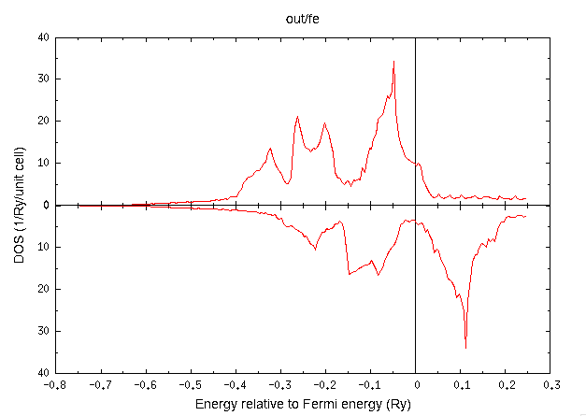
Then the total DOS of iron can be plotted as follows.
To plot the dispersion curve
Simply change the instruction in the first paragraph from a density of states (dos) command to an energy dispersion curve (spc) command.
c----------------------Fe------------------------------------
     spc   data/fe
c------------------------------------------------------------
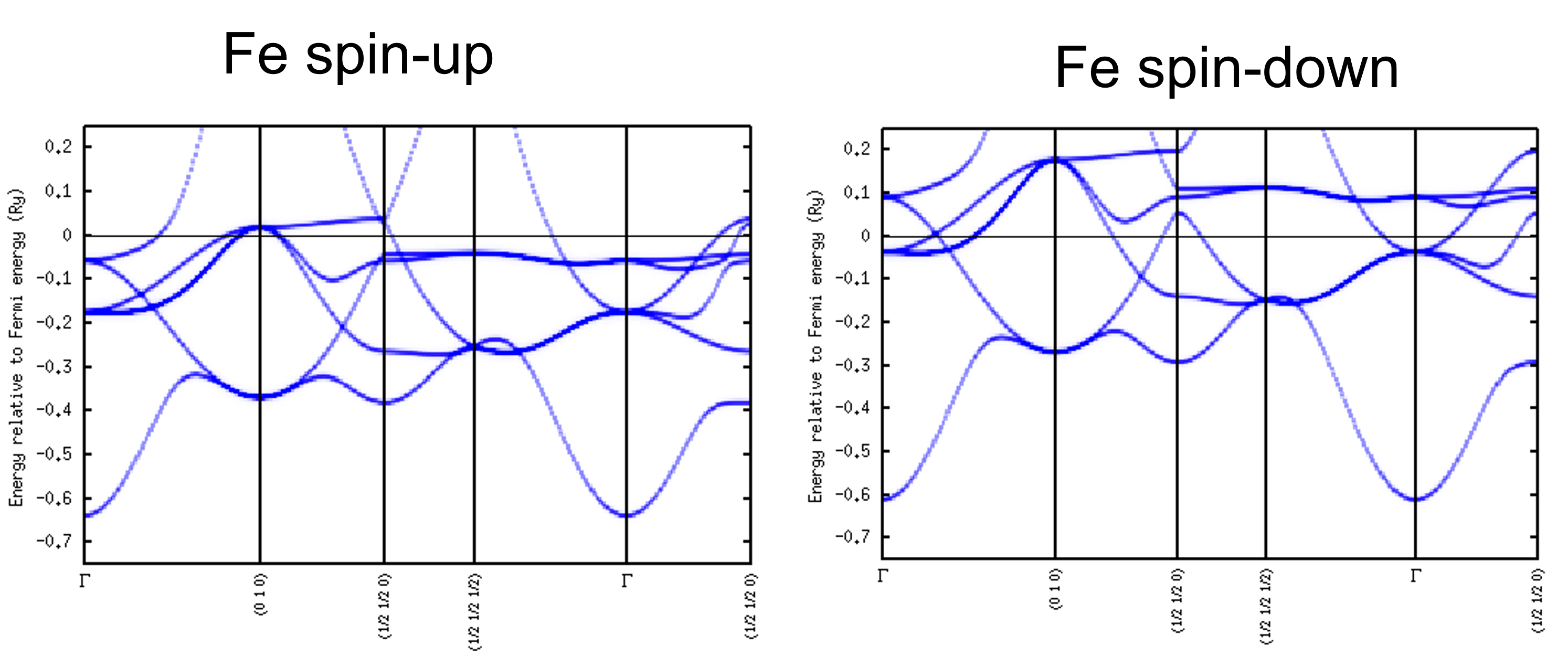
After running the calculation with the specx program, let’s plot the dispersion curve using a different plotting program than the one used to draw the DOS. The spc program also calls gnuplot to plot.
> spc data/fe_up.spc
> spc data/fe_dn.spc
Calculate different crystal structures
The input file for the case od cobalt
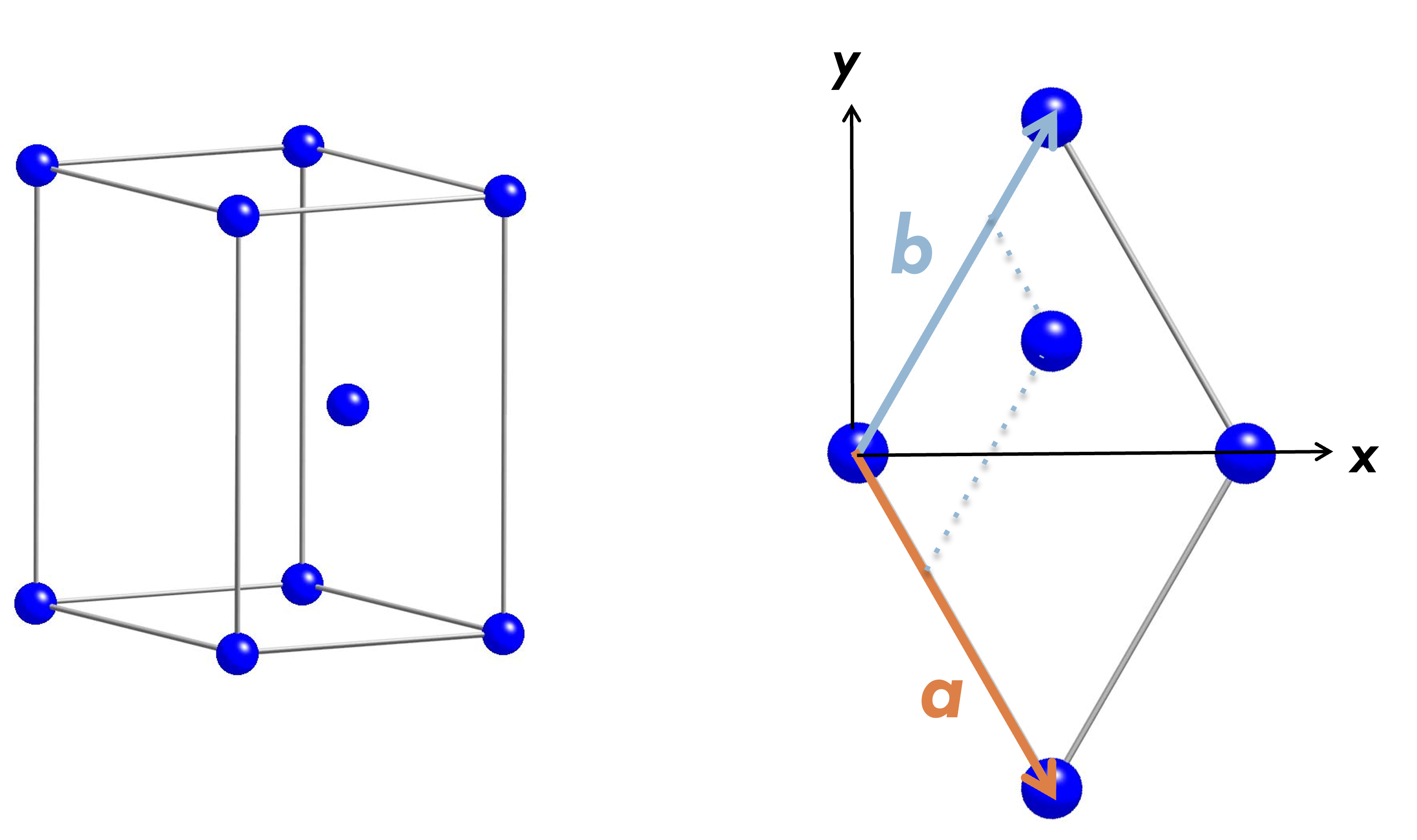
We want to do the calculations for cobalt, so we will present the hcp structure. The input file for the case of cobalt is also presented.
c----------------------Co------------------------------------
     go   data/co
c------------------------------------------------------------
c   brvtyp     a        c/a   b/a   alpha   beta   gamma
     hcp      4.74 , 1.6215 ,      ,      ,       ,      ,
c------------------------------------------------------------
c   edelt    ewidth    reltyp   sdftyp   magtyp   record
    0.001     1.0       nrl      mjw      mag      2nd
c------------------------------------------------------------
c   outtyp    bzqlty   maxitr   pmix
    update      4        50    0.023
c------------------------------------------------------------
c    ntyp
      1
c------------------------------------------------------------
c   type    ncmp    rmt    field   mxl  anclr   conc
    Co       1       1      0.0     2
                                          27    100
c------------------------------------------------------------
c   natm
     2
c------------------------------------------------------------
c   atmicx                        type
     0          0          0        Co
     0.5        0.86602    0.81075  Co
c------------------------------------------------------------
Here is a new way of expressing atomicx. The lower line shows the Cartesian coordinate system of the atomic positions in units of the lattice constant a. atomicx can also be expressed in fractions as follows.
c------------------------------------------------------------
c   atmicx                        type
     0          0          0        Co
     1/2        0.86602    0.81075  Co
c------------------------------------------------------------
Furthermore, the position can be specified using the unit lattice vectors a, b, and c. In this way, the atomic positions are specified by the orthogonal vectors of the three edges of a cuboid along x-, y-, and z-directions.
c------------------------------------------------------------
c   atmicx                        type
     0x         0y         0z       Co
     1/2x       0.86602y   1/2z     Co
c------------------------------------------------------------
Impurity problems
The Green’s function of the matrix is written as
 Let’s consider the scattering when one of the matrix atoms is replaced by an impurity atom.
CPA(Coherent potential approximation)
The macroscopic properties of substitutional disordered alloys are expressed as the result of configuration averaging with respect to atoms. We consider a t-matrix (coherent t-matrix, right figure below) corresponding to a virtual atom that reproduces the state after such a configuration averaging.
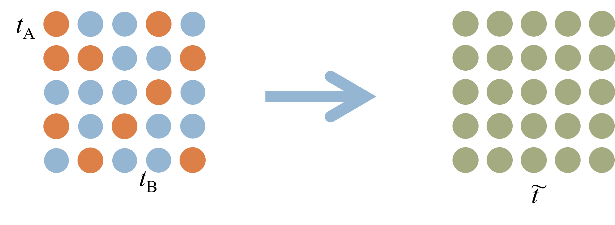
The coherent t-matrix satisfies the following relation.

It is a single-site approximation. Since the band calculation runs until the coherent potential is determined to be self-consistent, it takes longer than a normal electronic structure calculation.

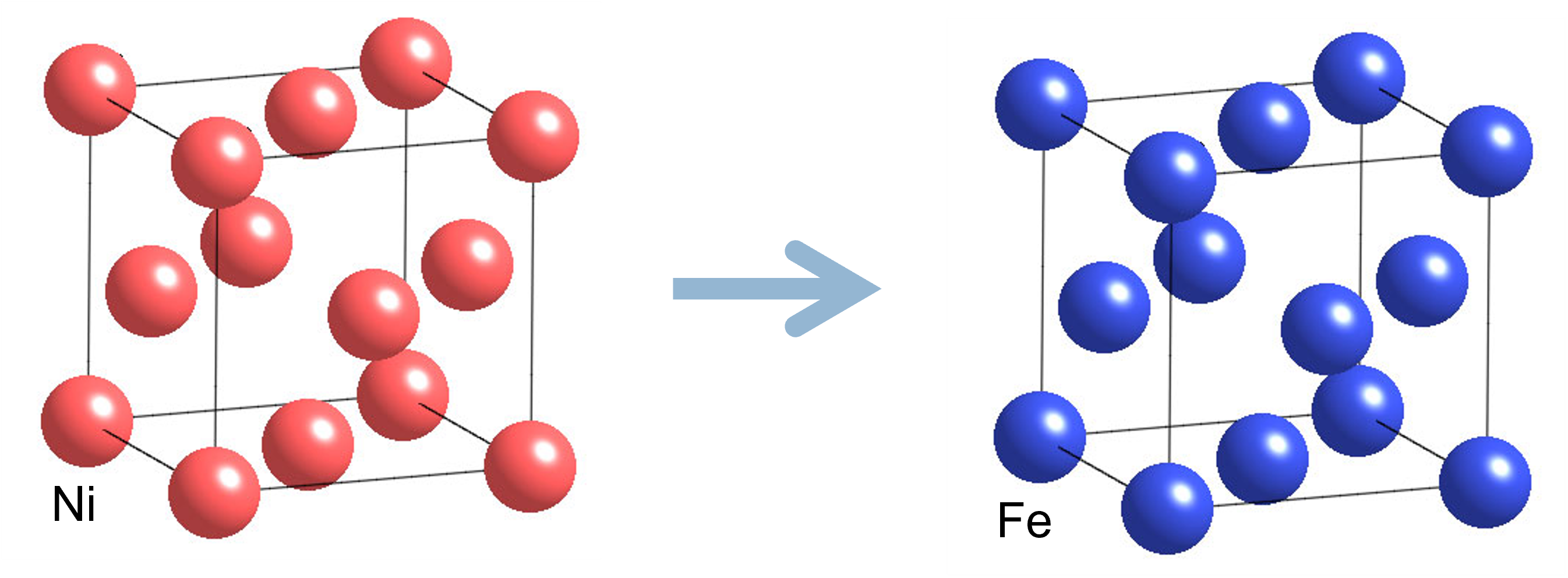
NiFe alloy(fcc)
The Ni atoms are replaced with Fe atoms.
We will calculate from nickel to the point where it becomes gamma iron.
The input file in the case of alloys would be, for example
c----------------------NiFe----------------------------------
     go   data/nife
c------------------------------------------------------------
c   brvtyp     a        c/a   b/a   alpha   beta   gamma
     fcc      6.55  ,      ,      ,      ,       ,      ,
c------------------------------------------------------------
c   edelt    ewidth    reltyp   sdftyp   magtyp   record
    0.001     1.0       nrl      mjw      mag      2nd
c------------------------------------------------------------
c   outtyp    bzqlty   maxitr   pmix
    update      4        50    0.023
c------------------------------------------------------------
c    ntyp
      1
c------------------------------------------------------------
c   type    ncmp    rmt    field   mxl  anclr   conc
    NiFe      2       1      0.0     2
                                          26     80
                                          28     20
c------------------------------------------------------------
c   natm
     1
c------------------------------------------------------------
c   atmicx                        type
     0          0          0        NiFe
c------------------------------------------------------------
type is the name of the type. ncmp is 2, indicating that there are two types of atoms occupying this type of position. The atom types anclr are Fe 26 and Ni 28.
The probabilities conc of atoms occupying this position are 80% and 20%, respectively. Let’s adjust this conc to calculate the various alloys.
Of course, there must be a correspondence between the two types (type and atmtyp in previous versions) that appear in two places.
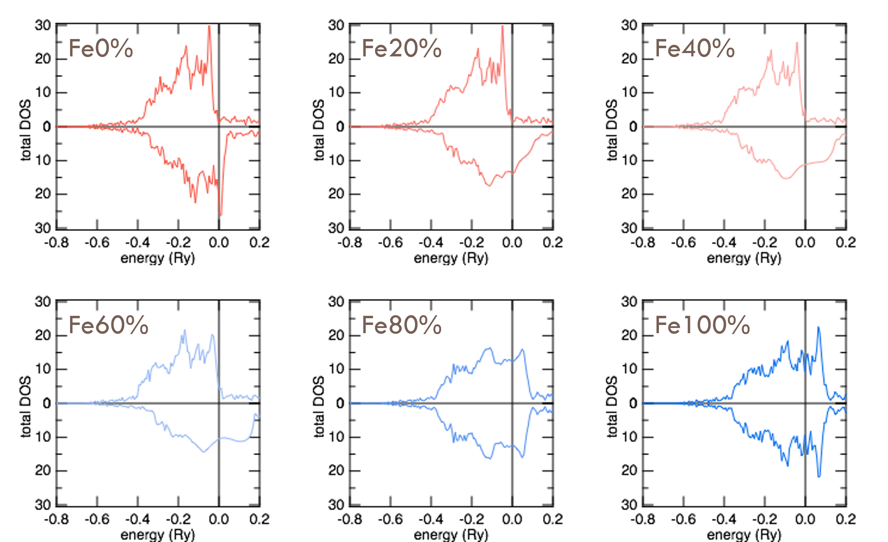
Plotting the total DOS for this alloy with varying percentages of Fe yields the following.
Slater-Pauling Curve
Let’s consider alloys composed of transition metal elements such as Fe, Co, and Ni.
The magnetic moments lie on a common curve.
The calculations reproduce the experimental results well, including the branching situation.
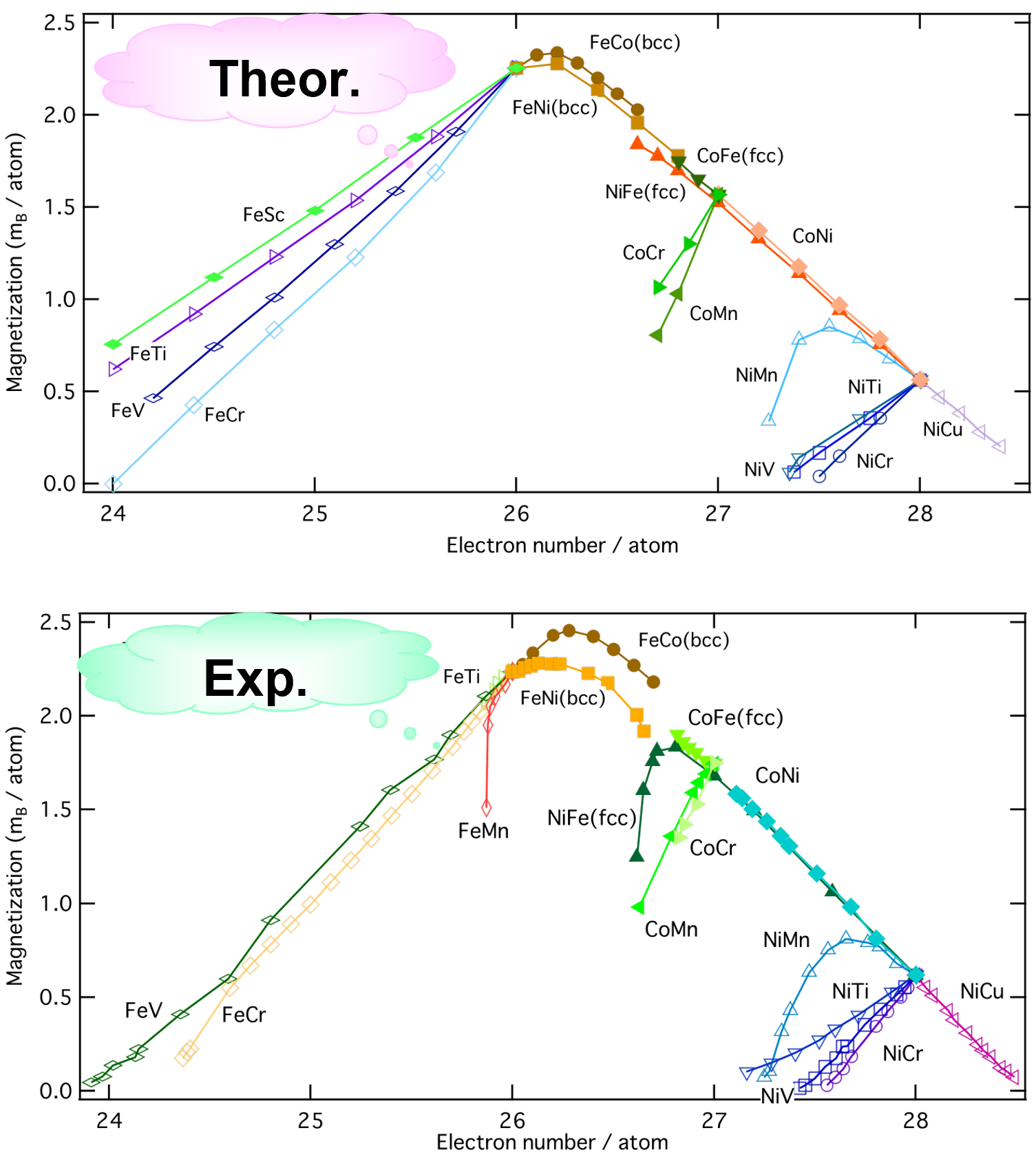
- H. Akai, Hyperfine Interactions 68 (1991) 3
- H.P.J. Wijn, Magnetic Properties of Metals (1991)
Input file for dispersion curve
c----------------------Inpurity inFe-------------------------
     go   data/feX
c------------------------------------------------------------
c   brvtyp     a        c/a   b/a   alpha   beta   gamma
     bcc      5.27  ,      ,      ,      ,       ,      ,
c------------------------------------------------------------
c   edelt    ewidth    reltyp   sdftyp   magtyp   record
    0.001     1.0       nrl      mjw      mag      2nd
c------------------------------------------------------------
c   outtyp    bzqlty   maxitr   pmix
    update      4        50    0.023
c------------------------------------------------------------
c    ntyp
      1
c------------------------------------------------------------
c   type    ncmp    rmt    field   mxl  anclr   conc
    FeX      2       1      0.0     2
                                          26    100
                                           1      0
c------------------------------------------------------------
c   natm
     1
c------------------------------------------------------------
c   atmicx                        type
     0          0          0        FeX
c------------------------------------------------------------
Looking at the lower part of conc, the probability (concentration) is zero.
References
- References
- 計算機ナノマテリアルデザイン入門(笠井秀明・赤井久純・吉田博編 大阪大学出版会)
- W.Kohn and N. Rostoker, Phys. Rev. 94 (1954) 1111.
- F.S. Ham and B. Segall, Phys. Rev. 124 (1961) 1786.
- H. Akai, J. Phys. Soc. Japan 51 (1982) 468.
- H. Akai, J. Phys.: Cond. Matter 1 (1989) 8045.
- KKR package http://kkr.issp.u-tokyo.ac.jp/